What does the Pythagorean Theorem have to do with machine learning? The Pythagorean Theorem is a formula to measure the hypotenuse of a triangle, which also allows us to calculate the distance between the origin and another point on a coordinate plane.
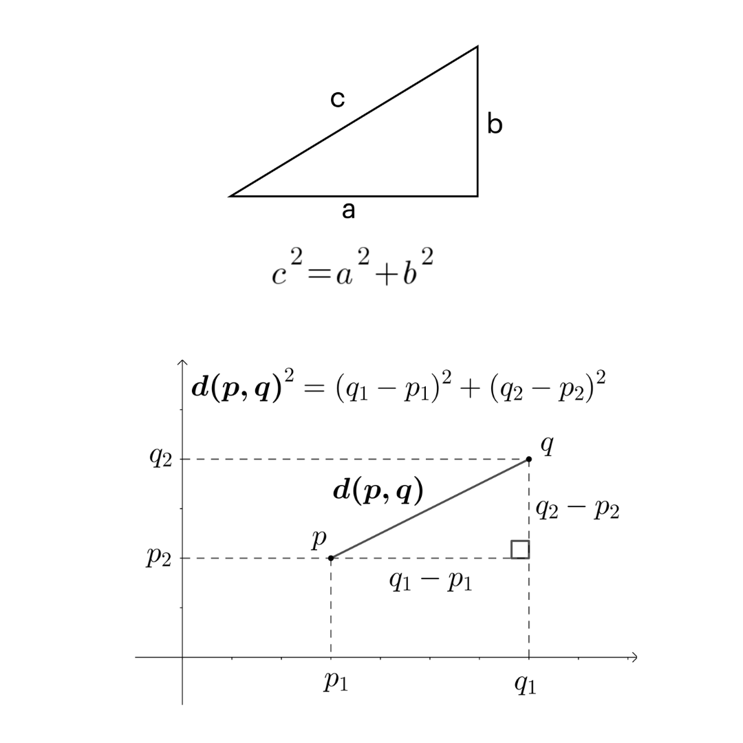
The Pythagorean Theorem can be rearranged to result in the Euclidean distance formula, to calculate the straight-line distance between any two points. The Euclidean distance metric is one of several distance metrics used in machine learning. One type of machine learning is clustering, where objects related to each other are grouped together. We can model how related objects are to each other by essentially assigning them to coordinates and calculating the distance between them; the further apart they are, the less related they are to each other.
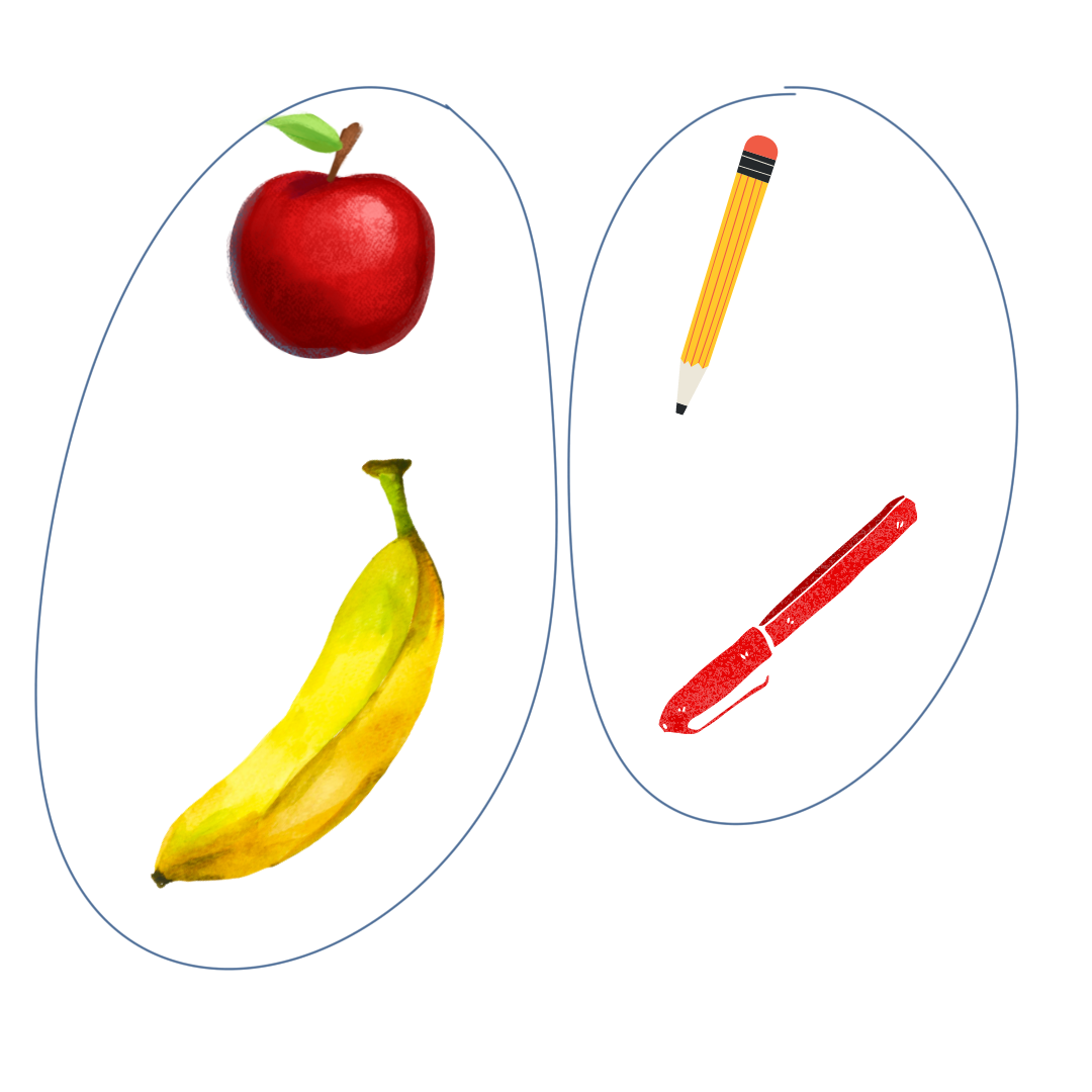
 Objects can be related to each other in many different aspects. For example, say you have a red apple, a banana, a red pen, and a Number 2 pencil. How would you group these objects into two groups? You could say the apple and banana go together because they are both fruits, and the pen and pencil go together because they are both writing instruments. But you could also say that the apple and pen should go together because they are both red, and the banana and the pencil should go together because they are both yellow. In this case, you could group by type of object or by color. Grouping by type of object might make more sense in this example.

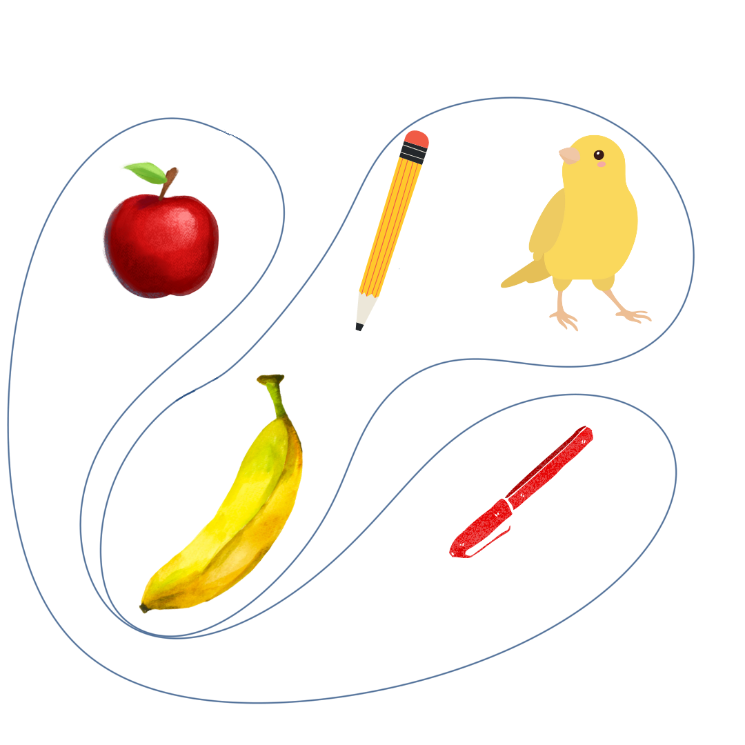
But what if we add in a canary to the things to be grouped? We want to make as many of the objects fit in the groups as possible, so the addition of a canary, which is yellow, would cause the grouping by color to make more sense.
In clustering, each of these objects would be a data point, and each aspect, such as type, color, size, and texture, would be a dimension of these objects. We call these different aspects features of the data. We can store this data in a matrix so that a computer can read and process the data.
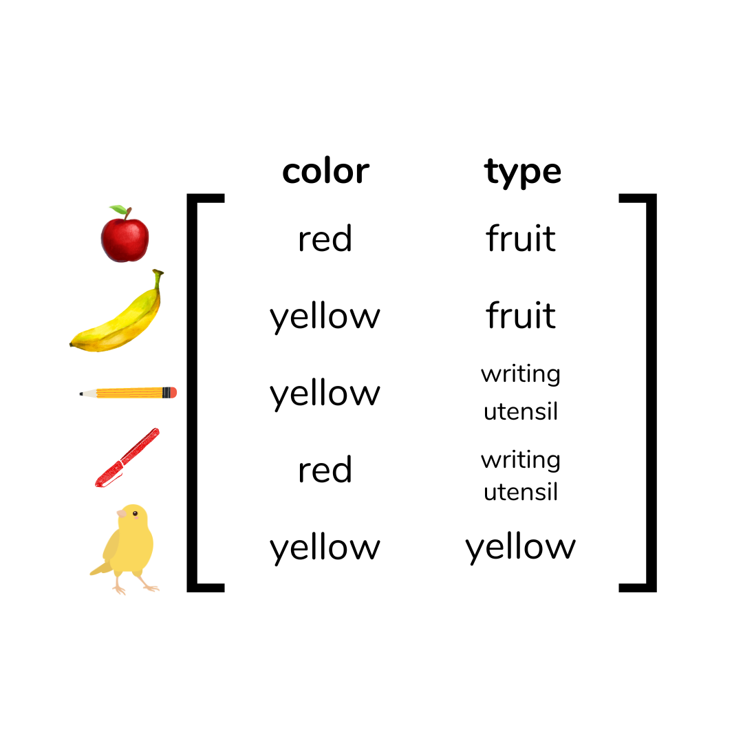
It might seem that if we add more features to the data, we would be able to group the objects better. Intuitively, we think we have more choices of what to group by. However, as we add more and more features, the majority of features would be irrelevant and actually make it more difficult to group. This is called noise in our model. For example, one feature of the data set we had earlier could be “does it have a beak?” But since the canary is the only object that has a beak, that doesn’t help us cluster the objects together. When considering the distance between data points, adding features adds a dimension to our model, which increases the distance between points. Also, adding “does it have a beak?” as a feature would actually just increase the amount of data we have to store, making our algorithms run slower.
When a computer clusters data points, points within the same cluster are similar and points in different clusters are not as similar. We quantify similarity using distance metrics. There are some properties of similarity that have to hold true for clustering to make sense:
- Symmetry: The distance from A to B is equal to the distance from B to A. This makes sense because if A is similar to B, B must be similar to A. Similarity goes both ways.
- Positive Separability: The distance from X to X is equal to 0, and the distance from X to any other point does not equal 0. This rule is needed because a data point cannot be different from itself, and if data points are different, they have to have a distance between them representing that difference.
- Triangle Separability: The distance from X to Y is less than or equal to the sum of the distance from X to Z and Y to Z. This makes sense because if Y is similar to Z, and X is similar to Z, then X must be similar to Y.

Euclidean distance is the straight-line distance from point A to point B, but here’s an example of another distance metric. Manhattan distance measures around blocks, resembling the route a car in a city would take around ceilings.
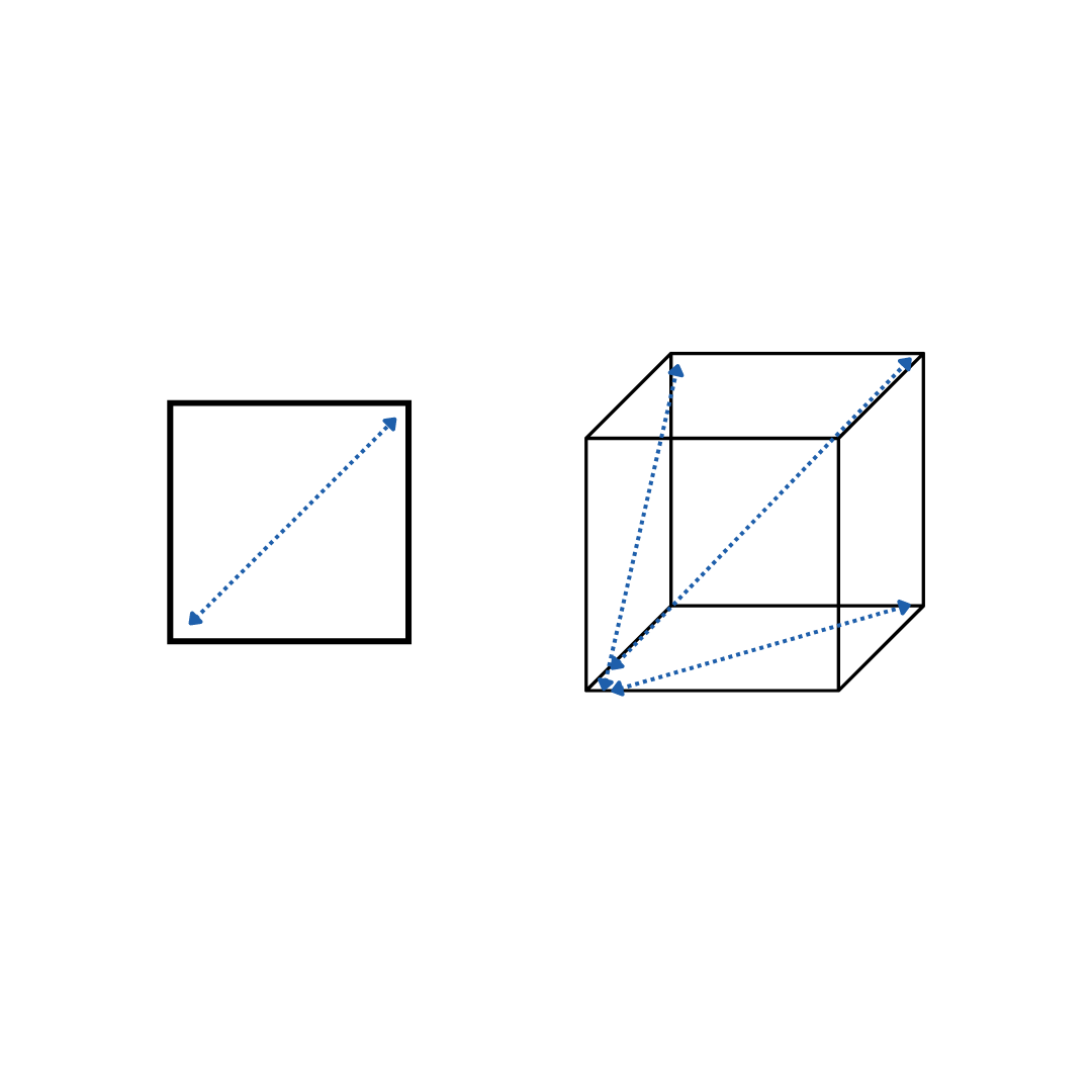
 An interesting phenomenon related to distance metrics is how they lose their meaning in higher dimensions. When we add features to our dataset and increase the number of dimensions, the average distance between points increases. Think about how in one dimension when we are looking at one feature, point A and B would be on a straight line, x units apart. But in two dimensions when we added another feature, if the second feature is just as far apart as the first for points A and B respectively, A and B would be sqrt(2)*x units apart. The same pattern continues when we add more and more dimensions.
As we increase dimensions and distance between points increases, the points also migrate towards the edges of the space. This is because the ratio of the limits of the space to the core of the space increases as the number of dimensions increases. Think about how a square with sides of length x has a perimeter of 4x and an area of x^2. A cube, on the other hand, with sides of length x has a surface area of 6x^2 and a volume of x^3. Let’s substitute 1 as x to compare these values.
Square perimeter = 4x = 4
Square area = x^2 = 1
Perimeter to area ratio = 4/1 = 4
Cube surface area = 6x^2 = 6
Cube volume = x^3 = 1
Surface area to volume area = 6/1 = 6
When the number of dimensions increased from 2 to 3, the ratio increased from 4 to 6. Once again, this pattern continues in higher dimensions.
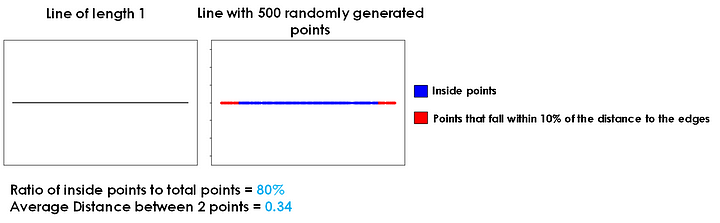
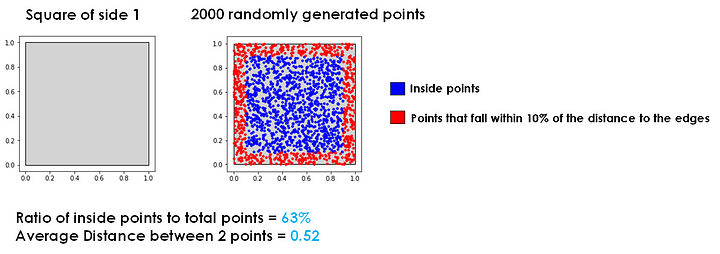
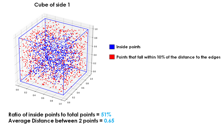
Let’s visualize a model with points randomly distributed around the model space.
In one dimension, approximately 20% of points will be within the outer 10% of the space. In two dimensions, approximately 37% of points will be within the outer 10% of the space. In three dimensions, approximately 49% of points will be within the outer 10% of the space.
Continuing on to dimensions of degrees that are essentially impossible for us to visualize, approximately 60% of points in four dimensions, 68% in five dimensions, 74% in six dimensions, and 80% in seven dimensions will be within the outer 10% of the space.
This concept brings us to the titular “infinitely-dimensional orange” concept; if we had an orange with infinity dimensions and points randomly distributed across the space, all the points would be on the peel of the orange, with no points spread around in the interior.

Using more features allows each data point to become more different from each other, which makes them more sparsely distributed. This makes it harder to cluster the points accurately! In machine learning models, we address this issue using feature selection and dimensionality reduction techniques to find the most relevant features and reduce the number of dimensions we utilize to cluster data points. Not only does this reduce the processing power a computer would need to run the algorithm, but accuracy in clustering generally also increases by preventing the “infinitely-dimensional orange” phenomenon.
Reference
- https://towardsdatascience.com/the-surprising-behaviour-of-distance-metrics-in-high-dimensions-c2cb72779ea6
- Georgia Tech CS 4641 lecture slides by Professor Roozbahani