An Infinitely Dimensional Orange: A Slice of Machine Learning

What does the Pythagorean Theorem have to do with machine learning? The Pythagorean Theorem is a formula to measure the hypotenuse of a triangle, which also allows us to calculate the distance between the origin and another point on a coordinate plane.
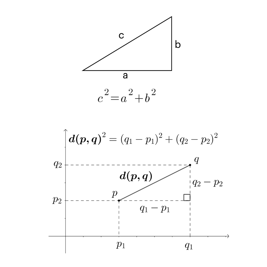
The Pythagorean Theorem can be rearranged to result in the Euclidean distance formula, to calculate the straight-line distance between any two points. The Euclidean distance metric is one of several distance metrics used in machine learning. One type of machine learning is clustering, where objects related to each other are grouped together. We can model how related objects are to each other by essentially assigning them to coordinates and calculating the distance between them; the further apart they are, the less related they are to each other. 

Objects can be related to each other in many different aspects. For example, say you have a red apple, a banana, a red pen, and a Number 2 pencil. How would you group these objects into two groups? You could say the apple and banana go together because they are both fruits, and the pen and pencil go together because they are both writing instruments. But you could also say that the apple and pen should go together because they are both red, and the banana and the pencil should go together because they are both yellow. In this case, you could group by type of object or by color. Grouping by type of object might make more sense in this example.
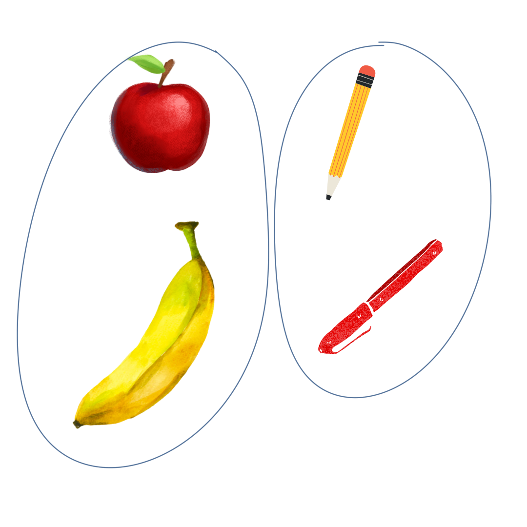
But what if we add in a canary to the things to be grouped? We want to make as many of the objects fit in the groups as possible, so the addition of a canary, which is yellow, would cause the grouping by color to make more sense.

In clustering, each of these objects would be a data point, and each aspect, such as type, color, size, and texture, would be a dimension of these objects. We call these different aspects features of the data. We can store this data in a matrix so that a computer can read and process the data.
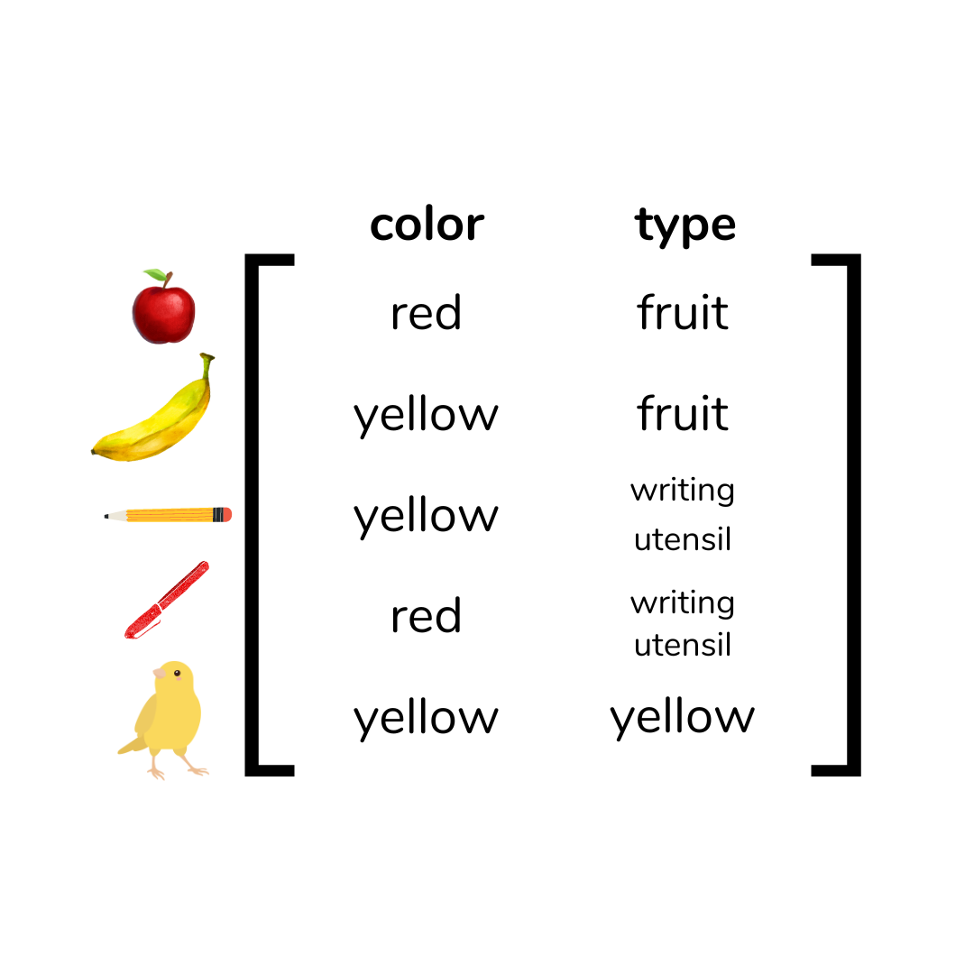
It might seem that if we add more features to the data, we would be able to group the objects better. Intuitively, we think we have more choices of what to group by. However, as we add more and more features, the majority of features would be irrelevant and actually make it more difficult to group. This is called noise in our model. For example, one feature of the data set we had earlier could be “does it have a beak?” But since the canary is the only object that has a beak, that doesn’t help us cluster the objects together. When considering the distance between data points, adding features adds a dimension to our model, which increases the distance between points. Also, adding “does it have a beak?” as a feature would actually just increase the amount of data we have to store, making our algorithms run slower.
When a computer clusters data points, points within the same cluster are similar and points in different clusters are not as similar. We quantify similarity using distance metrics. There are some properties of similarity that have to hold true for clustering to make sense:

  • Symmetry: The distance from A to B is equal to the distance from B to A. This makes sense because if A is similar to B, B must be similar to A. Similarity goes both ways.
  • Positive Separability: The distance from X to X is equal to 0, and the distance from X to any other point does not equal 0. This rule is needed because a data point cannot be different from itself, and if data points are different, they have to have a distance between them representing that difference.
  • Triangle Separability: The distance from X to Y is less than or equal to the sum of the distance from X to Z and Y to Z. This makes sense because if Y is similar to Z, and X is similar to Z, then X must be similar to Y.

Euclidean distance is the straight-line distance from point A to point B, but here’s an example of another distance metric. Manhattan distance measures around blocks, resembling the route a car in a city would take around ceilings. 

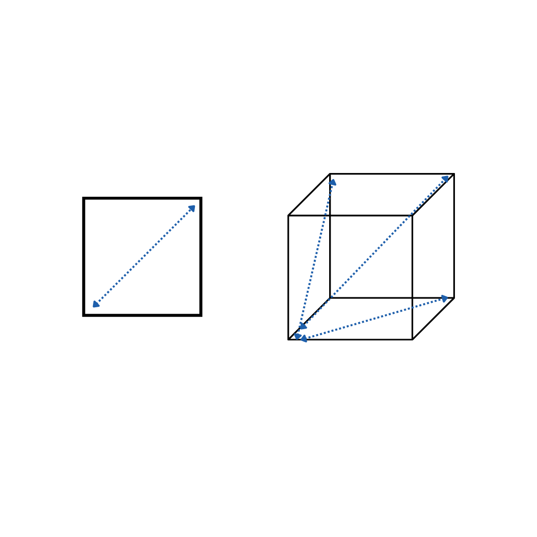
An interesting phenomenon related to distance metrics is how they lose their meaning in higher dimensions. When we add features to our dataset and increase the number of dimensions, the average distance between points increases. Think about how in one dimension when we are looking at one feature, point A and B would be on a straight line, x units apart. But in two dimensions when we added another feature, if the second feature is just as far apart as the first for points A and B respectively, A and B would be sqrt(2)*x units apart. The same pattern continues when we add more and more dimensions.

As we increase dimensions and distance between points increases, the points also migrate towards the edges of the space. This is because the ratio of the limits of the space to the core of the space increases as the number of dimensions increases. Think about how a square with sides of length x has a perimeter of 4x and an area of x^2. A cube, on the other hand, with sides of length x has a surface area of 6x^2 and a volume of x^3. Let’s substitute 1 as x to compare these values. 

Square perimeter = 4x = 4

Square area = x^2 = 1

Perimeter to area ratio = 4/1 = 4

Cube surface area = 6x^2 = 6

Cube volume = x^3 = 1

Surface area to volume area = 6/1 = 6

When the number of dimensions increased from 2 to 3, the ratio increased from 4 to 6. Once again, this pattern continues in higher dimensions.

Let’s visualize a model with points randomly distributed around the model space.

In one dimension, approximately 20% of points will be within the outer 10% of the space. In two dimensions, approximately 37% of points will be within the outer 10% of the space. In three dimensions, approximately 49% of points will be within the outer 10% of the space.
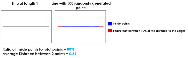
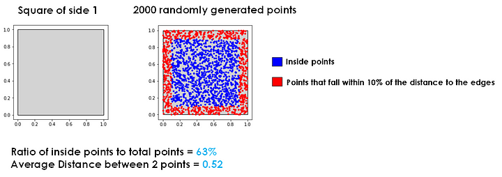
Continuing on to dimensions of degrees that are essentially impossible for us to visualize, approximately 60% of points in four dimensions, 68% in five dimensions, 74% in six dimensions, and 80% in seven dimensions will be within the outer 10% of the space.
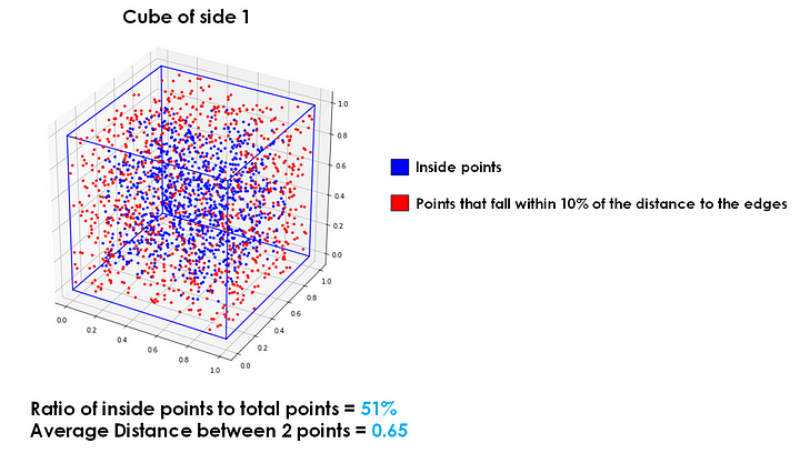
This concept brings us to the titular “infinitely-dimensional orange” concept; if we had an orange with infinity dimensions and points randomly distributed across the space, all the points would be on the peel of the orange, with no points spread around in the interior.

Using more features allows each data point to become more different from each other, which makes them more sparsely distributed. This makes it harder to cluster the points accurately! In machine learning models, we address this issue using feature selection and dimensionality reduction techniques to find the most relevant features and reduce the number of dimensions we utilize to cluster data points. Not only does this reduce the processing power a computer would need to run the algorithm, but accuracy in clustering generally also increases by preventing the “infinitely-dimensional orange” phenomenon.

Reference

Your journey starts here! Let’s talk!

ThemeRex © 2026. All rights reserved.
  Timothy Durham was convicted of rape when a test showed his DNA genotype matched the DNA recovered from the crime scene. Eye witnesses testified that Durham was in a different state at the time of the incident, but he wasn’t exonerated from his 3000 year sentence until follow up DNA analysis showed that the preliminary forensic analysis used in the trial was misinterpreted (Thomas et al.). DNA testing serves an invaluable part in our criminal justice system, but it comes with complications and bias that can lead to wrongful convictions and misinformed juries.  

Background:

Forensic genetics aims to identify the origin of a biological sample. It can be traced back to Karl Landsteiner who discovered human ABO blood groups. With blood groups, suspects could be eliminated based on their blood type. For example, if a suspect had type A blood and there was type B blood left at the scene by the perpetrator, the investigators could rule out the suspect. Unfortunately, the reverse didn’t work. If the suspect and perpetrator both had the same blood type, it can’t be concluded that the suspect was guilty. Blood identifiers evolved into 8 distinct categories which improved the ability to eliminate suspects, but could only conclude that (if the system matched) it might be the perpetrator or this person might be related to the perpetrator (Jobling and Gill). The field evolved in the 1980s with the discovery of Minisatellites, lines of repetitive DNA that don’t encode proteins. Minisatellite patterns in DNA create what we know today as the DNA fingerprint, and it has a much higher accuracy rate than previous methods (Augustyn et al.). Around the same time, a breakthrough for victims of sexual assault was discovered. In the case of assault, bodily fluids of both the victim and the assaulter can get mixed. A process called differential lysis was created which could selectively increase the concentration of sperm in a fluid sample thereby allowing for accurate DNA testing (Jobling and Gill). Forensics evolved to use single-locus probe testing after several years because of its ease of interpretation. It looked at specific minisatellites that had high variability between subjects. This was the first DNA-based method to be used in a criminal investigation. Two murder homicides from several years apart were connected using DNA evidence. The evidence was then used to exonerate an innocent man, and the guilty party was found when he tried to evade mandatory DNA testing for all men in the small town. His guilt was then reinforced when the DNA profiles matched, and he gave a confession (Jobling and Gill). Finding DNA at a crime scene doesn’t guarantee that you’ll find a murderer. There are issues with non-pure samples and limited samples that make DNA work difficult, and accreditation of facilities and new techniques and take time (Jobling and Gill).  

Subjectivity of DNA Interpretation:

In a 2009 publication, the National Academy of Science discusses the possibility for subjective influence in lab based forensics. The interpretation bias happens in complex cases where, for example, there could be a mixture of DNA. A study published in 2011 looked specifically at this issue. A gang rape happened in Georgia, and the mixture in DNA from the case was used to prosecute one suspect after another suspect took a plea bargain to testify against him. With DNA mixtures, there are three possible conclusions: suspect excluded, suspect cannot be excluded, and inconclusive. If the suspect is excluded, it means that there’s little to no possibility that his DNA is part of the sample. If the suspect cannot be excluded, it means that there’s a possibility that his DNA is part of the sample. In the trial, the DNA examiners who knew the context of the case concluded that the suspect being prosecuted could not be excluded. The 2011 study gave the DNA evidence from this case and the DNA profiles of the suspects to 17 forensic examiners. These examiners had no context of the case, and they all worked independently. Of the 17, only 1 came to the same conclusion (suspect cannot be excluded) as the examiners who knew the context of the case. Twelve of the 17 concluded that the suspect who was prosecuted and convicted had no relation to the DNA found in the sample. Not only does this show that subjectivity occurs due to the context of the case, but the 17 examiners came up with different findings based on their past experiences meaning that not all DNA analysis is objective. Some organizations like the Scientific Working Group on DNA Analysis Methods say that quantitative statistical evidence should be presented with every categorical conclusion, but the US doesn’t require this (Dror and Hampikian).

False Positives:

There are two categories that cause wrongful identification in a DNA report: coincidental matches and false positives. Coincidental matches are DNA matches between two unrelated people. The probability of these matches is about 1 to 500,000 for white individuals and about 1 to 350,000 for black individuals. This small probability of coincidental matches makes people feel confident in DNA evidence. False positives, on the other hand, are matches between DNA and test DNA that result from issues in the forensics lab. There have been multiple cases of forensics labs accidentally switching victim and suspected rapist DNA which lead to convictions that were later overturned when the lab realized the error. There are also cases of misreading or misunderstanding a sample. In a case from 1993, a man was convicted of rape because someone interpreted a mixed sample of victim and perpetrator DNA as an individual sample. The conviction was again overturned. To prevent false convictions, retesting DNA is allowed, but it’s not an efficient solution. Many people are pushing for statistical information on the probability of false positives, so that the jurors can make accurate judgements based on DNA evidence (Thomas et al.).  

Conclusion:

DNA analysis is a useful tool for the criminal justice system, but subjectivity can be an issue in forensic testing. To combat wrongful convictions, there are organizations like The Innocence Project who use DNA testing to free the innocent, but reformed forensic testing standards should be put in place to prevent subjectivity and to ensure juries are correctly informed during trials. https://www.innocenceproject.org/    

Citation:

Augustyn , Adam, et al. “DNA Finerprinting.” Encyclopedia Britannica , 26 Apr. 2018, www.britannica.com/science/DNA-fingerprinting#ref153186. Dror, Itiel E., and Greg Hampikian. “Subjectivity and Bias in Forensic DNA Mixture Interpretation.” Science & Justice, vol. 51, no. 4, 2011, pp. 204–208., doi:10.1016/j.scijus.2011.08.004. Jobling, Mark A., and Peter Gill. “Encoded Evidence: DNA in Forensic Analysis.” Nature Reviews: Genetics, vol. 5, no. 10, Oct. 2004, pp. 739–751., doi:10.1038/nrg1455. Thompson, William C, et al. “How the Probability of a False Positive Affects the Value of DNA Evidence.” Journal of Forensic Sciences, vol. 48, no. 1, Jan. 2003, pp. 1–8., doi:10.1520/jfs2001171.